Projective Varieties

Your web browser must have JavaScript enabled in order for this application to display correctly.

What's going on here?

Many of the well known algebraic surfaces are defined in projective space $\mathbb{P}^3$ for example the Fermat Cubic is defined as $x^3+y^3+z^3+w^3=0$ yet most images just show a projection obtained by setting $w=1$ and projecting into $\mathbb{R}^3$ giving the surface defined by $x^3+y^3+z^3+1=0$. To draw pictures of this surface we normally take a finite domain, which may miss off important details, which lie at infinity, i.e. points where $w=0$.

Here we calculate the surface in four separate parts which cover all of $\mathbb{P}^3$ and then use Stereographic projection to project the whole surface to the inside of a sphere. No parts of the surface is missed in this projection.

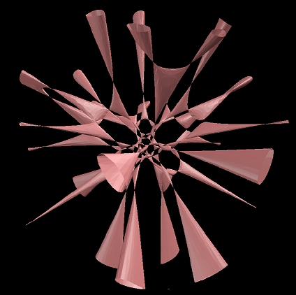
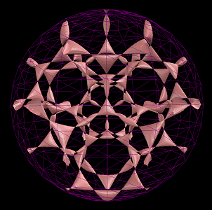
In the above figure of Sarti's Octic with 144 nodes, the typical projection on the left does not show the full set of 144 nodes. The stereographic projection on the right displays all the nodes. Whilst stereographic does not preserve straight line it keeps the distances between nodes relatively similar.

Understanding projective space

Lets start with the 2D example, here projective space can be thought of as set of all possible lines in the plane. The typical equation to define a line, $y = m x + c$. This equation covers most, but not all, lines. It excludes vertical lines defined by $x = c$. So if we want to describe the set of all possible lines we can take the set of regular lines, given by all points $(m,c)$ and add on the set of irregular lines $(c)$. Hence, we have the Euclidean plane $\mathbb{R}^2$ with and extra "line at infinity" $\mathbb{R}$. Taken together these make the real projective plane $\mathbb{P}^2$.

A better way to describe this space is using $a x + b y + c = 0$ as the equation of a line, and taking the set of all possible values $(a,b,c)$. This set can describes all possible lines, setting $a=m, b=-1$ gives the normal $y = m x + c$ equation, and setting $a=1, b=0$ gives the vertical lines, $x=c$. This set has multiple elements describing the same line, $2 a\, x + 2 b\, y + 2 c = 0$ gives exactly the same line as $a\, x+b\,y+x=0$, indeed for any non zero multiple $\lambda\ne 0$ we have $\lambda a\, x + \lambda b\, y + \lambda c = 0$ describes the same line. All these equivalent points are identified by using homogeneous coordinates written as $(a:b:c)$ with the equivalence relation $(\lambda a: \lambda b: \lambda c) = (a : b : c)$, for any $\lambda\ne 0$. This set defines the real projective plane $\mathbb{P}^2$.

Another way the think about the space is as the set of all lines through the origin in $\mathbb{R}^3$. Any such line could be describes by a point $(a,b,c)$ on the line, and any non-zero multiple of the point $(\lambda a, \lambda b, \lambda c)$ specifies the same line. In other dimensions we have the table:

Ways of thinking about Real Projective Spaces
Name	Real projective line	Real projective plane	Real projective 3-space
Symbol	$\mathbb{P}^1$	$\mathbb{P}^2$	$\mathbb{P}^3$
Description		Set of all lines in the plane	Set of all planes in 3-space
Description	Set of lines through the origin in $\mathbb{R}^2$	Set of lines through the origin in $\mathbb{R}^3$	Set of lines through the origin in $\mathbb{R}^4$
Coordinates	$(x:y)$	$(x:y:z)$	$(x:y:z:w)$

Projecting to Euclidean space

There are several ways we can construct a projection from $\mathbb{P}^2$ to the Euclidean plane $\mathbb{R}^2$. One is to divide by one of the coordinates, say $(x:y:z) \to (x/z, y/z) $. If $z=1$ this map simply becomes $(x:y:1) \to (x, y) $, this map sends those points where $z=0$ to infinity, and we call $z=0$ the line at infinity. Thinking of real projective space as the set of lines through the origin this then the projection yields the intersection of the lines with the plane $z=1$. Many other projections can be obtained by first rotating in $\mathbb{P}^2$ and then projecting. So for example we could have the rotation $(x:y:z)\to(x:-z:y)$ followed by a projection giving the map $(x:y:z)\to(x/y,-z/y)$.

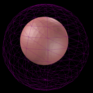
If we consider a sphere $x^2+y^2+z^2=1$, each line through the origin cuts the sphere in two points, $(x,y,z)$ and $(-x,-y,-z)$ so we can model $\mathbb{P}^2$ as the lower half sphere, $x^2+y^2+z^2=1,z<=0$. Then we can use stereographic projection to map this inside of the circle in $\mathbb{R}^2$. This is a central projection from the point $(0,0,1)$ on to the plane $z=-1$. Which gives the map $(x,y,z)\to\frac{2}{1-z}(x,y)$.

We can illustrate these by considering the 1D dimensional case. Here the projective space $\mathbb{P}^1$ consists of the set of lines in $(x-z)$ plane which pass through the origin. We can find the perspective-projection of this space by taking the points where these lines intersect the line $z=-1$. For the stereographic first take the intersections with the lower half of the unit sphere, and then project from the from the point $(0,1)$ onto the plane $z=-1$. This projection always give points lying between -2 and 2, the thin dotted lines show the boundary of this set.

Projection from RP^2 to R — Three lines $A, B, C$ lines through the origin and their images $a, b, c$ under perspective projection (left), their intersections with the lower half of the unit sphere, $a', b', c'$, and their stereographic projections $a'', b'', c''$.

Stereographic projection from RP^2 to R — Three lines $A, B, C$ lines through the origin and their images $a, b, c$ under perspective projection (left), their intersections with the lower half of the unit sphere, $a', b', c'$, and their stereographic projections $a'', b'', c''$.

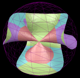
Going up a dimension a stereographic projection of $\mathbb{P}^2$ gives points inside a circle and stereographic projection of $\mathbb{P}^3$ gives points inside a sphere.

One interesting property of projective spaces is they are non-oriented. In the stereographic projection points on the boundary are identified with their antipodal point. We will see the effect of this when consider rotating the surface.

Varieties in projective space

Curves and surfaces can be defined by equations in the coordinates. For example a line in $\mathbb{P}^2$ can be defined by $x+y+z=0$. Consider as set in $\mathbb{R}^3$ this is a plane through the origin, but's its perspective projection is a line. Stereographic projection gives the same topological structure but looses metrical properties and maps straight lines to circles.

Such equations must be Homogeneous function where each term has the same degree. Scaling each coordinate by the constant will not change the surface, so $2 x+2 y+2 z=0$ give the same set as $x+y+z=0$. Likewise in quadratic like $x^2 - y z=0$ each term as degree two. This describes a cone in $\mathbb{R}^3$ and a conic when projected to $\mathbb{R}^3$. Multiplying each coordinate by two gives $(2 x)^2- (2 y)(2 z) = 4 x^2 - 4 y z = 0$ the same set.

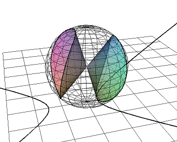
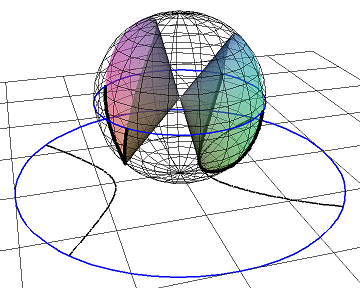
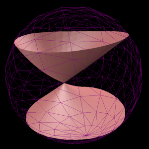
In the diagram below we have a different quadratic, $0.7 x^2 - y^2 - 0.2 y^2 + 0.5 x z$ in $\mathbb{P}^2$, this forms a cone which intersect the unit sphere in two identical curves, which are inversions of each other. Projecting the curve from the origin onto the plane $z=-1$ gives a curve with branches will goes off to infinity and come on the other side, for the cone this is a hyperbola. Using a stereographic projection gives a curve contained inside the blue circle. The points where the curve touch the circle should be identified with their diametrically opposite points. 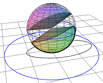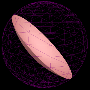Rotating the cone changes the image, and can be changed from one with two branches to a single closed curve. This shows that in projective spaces there is no difference between ellipses and hyperbola.

Projection of a cone in RP^3 to plane — A cone $0.7 x^2 - y^2 - 0.2 y^2 + 0.5 x z$ in $\mathbb{P}^2$, its intersection with the unit sphere, and its perspective projection to the plane (left), stereographic projection (middle) and a rotated version of the cone.

Stereographic projection of a cone in RP^3 to plane — A cone $0.7 x^2 - y^2 - 0.2 y^2 + 0.5 x z$ in $\mathbb{P}^2$, its intersection with the unit sphere, and its perspective projection to the plane (left), stereographic projection (middle) and a rotated version of the cone.

Surfaces in $\mathbb{P}^3$

In $\mathbb{P}^3$ surfaces are defined by equations in four homogeneous coordinates, so $x+y+z+w=0$ describes a plane. A c projection will be slightly distorted, forming part of a sphere. For degree 2 we can have ellipsoids, cones, and hyperbolids. Ellipsoids can appear either as a single closed surface or as a surface with two components depending on the rotation.

Stereographic projection of a plane — A plane $x + y + z + w$ in $\mathbb{R}^2$, ellipsoid $x y-x z+x w+y z-y w+z w$ (two views), cone $x y-x z+x w+y z-y w$ and hyperboloid $x y-x z+x w+y z+y w+z w$.

Stereographic projection of a cone — A plane $x + y + z + w$ in $\mathbb{R}^2$, ellipsoid $x y-x z+x w+y z-y w+z w$ (two views), cone $x y-x z+x w+y z-y w$ and hyperboloid $x y-x z+x w+y z+y w+z w$.

In degree three the Clebsch_surface is defined as $x^{3}+y^{3}+z^{3}+w^{3}=(x+y+z+w)^{3}$ and all terms are cubic. Projection of this set onto the space $w=1$ yield a polynomial where the terms a have varying degrees $$\begin{align}3(x^2 y&+xy^2+ x^2 z+x z^2+y^2 z+yz^2)+6xyz\\&+3(x^2+y^2+z^2)+6(xy+xz+yz)+3(x+y+z)\end{align}$$

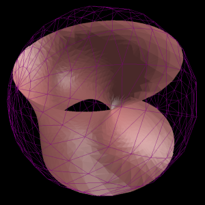
loosing some of the algebraic symmetry.

Calculation

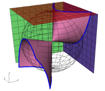
Its not possible to calculate surfaces directly in $\mathbb{P}^3$ all it possible to do is calculate algebraic surfaces in finite regions of Euclidean space $\mathbb{R}^3$. Taking just one slice through like $w=1$ will not find the whole surface. So multiple slices are taken. In the case of $\mathbb{P}^2$ we can find the intersection of a surface $f(x,y,z)=0$ with the three faces of the surrounding cube, $\{x\in[-1,1], y\in[-1,1], z=1\}$, $\{x\in[-1,1], y=1, z\in[-1,1]\}$ and $\{x=1, y\in[-1,1], z\in[-1,1]\}$. This involves calculating the three curves $f(x,y,1)=0$, $f(x,1,y)=0$ and $f(1,y,z)=0$. The three intersections can then be projected onto a plane using either perspective of stereographic projection. As antipodal points are identified there is no need to calculate intersections with the other three faces.

For surfaces $f(x,y,z,w)=0$ in $\mathbb{P}^3$ the intersection with four cubes are calculated $\{x\in[-1,1], y\in[-1,1], z\in[-1,1], w=1\}$, $\{x\in[-1,1], y\in[-1,1], z=1, w\in[-1,1]\}$, $\{x\in[-1,1], y=1, z\in[-1,1], w\in[-1,1]\}$ and $\{x=1, y\in[-1,1], z\in[-1,1], w\in[-1,1]\}$.

A cubic showing separate colours for each the four surfaces calculated, these surfaces knit together to create the complete surface

The full algorithm is:

Calculate the sets $\{f(x,y,z,1) : x\in[-1,1], y\in[-1,1], z\in[-1,1] \}$, $\{f(x,y,1,w) : x\in[-1,1], y\in[-1,1], w\in[-1,1] \}$, $\{f(x,1,z,w) : x\in[-1,1], z\in[-1,1], w\in[-1,1] \}$ and $\{f(1,y,z,w) : y\in[-1,1], z\in[-1,1], w\in[-1,1] \}$;
Rotate in $\mathbb{R}^4$;
Cut each surface into sets $\{x,y,z,w:w>0\}$, $\{x,y,z,w:w<0\}$;
Project into $\mathbb{R}^3$, using either perspective of stereographic projections;
For perspective projection clip the result.

The four dimensional rotation is applied by using three rotation matrices $$R_{xw}=\begin{pmatrix}\cos \theta& 0 & 0 &\sin \theta\\0 & 1 & 0 & 0\\0 & 0 & 1 & 0\\ -\sin \theta & 0 & 0 & \cos \theta\end{pmatrix},$$ $$R_{yw}=\begin{pmatrix}1 & 0 & 0 & 0\\0 & \cos \theta& 0 &\sin \theta\\0 & 0 & 1 & 0\\ 0 & -\sin \theta & 0 & \cos \theta\end{pmatrix},$$ $$R_{zw}=\begin{pmatrix}1 & 0 & 0 & 0\\0 & 1 & 0 & 0\\ 0 & 0 & \cos \theta &\sin \theta\\ 0 & 0 & -\sin \theta & \cos \theta\end{pmatrix}$$ and their inverses, for some small fixed angle $theta$. The actual rotation matrix $M$, is incrementally adjusted say applying $M=R_{xw} M$ when the Rxw+ button is pressed. Applying the $R_{xw}$ matrix gives the effect of shifting the surface in the positive x direction.